Draft Player Comparison Tool *Updated for 2008-2012*

Updated 9/16/16 to include 2008-2012 Drafts 

Hello all,

Previously, I provided a draft comparison tool to allow you to compare players in the 2016 draft based on salary.  The thought behind this was, "If player X is slotted to be awarded a $20MM contract and player Y a $4MM deal, than player X should be 5 times as valuable to his team as player Y."
Looking at a fresh draft is nice, but we won't know what those values mean for a few years.  So, I've decided to update the table to reflect on the 2008-2012 drafts, as those players can be considered mature.

Follow the link below to the spreadsheet.  There, you willl find two tabs:

Draft Class

This tab lists the draftees in order of selection and the slotted contract value for each based on draft position/  We used the 2014 rookie contract scale for convenience, but remember, this is a relative comparison tool, so the values of the contracts are not important, just the scale.  It is helpful to sort by position so you can easily compare QBs, OTs or any other position.  You can even compare players at different positions.

Comparison Tool

This engine will allow you to compare any two players in the draft and get an idea of relative value.  The list of players is to the left of the drop down windows. 

I hid the built in player value comparisons that compared each player's value to the #1 overall pick, the #1 player at his position and the player at his position drafted directly before him.  I found them interesting but thought perhaps all the extra numbers just cluttered up the spreadsheet.  If you would like them returned, let me know.

Here are a couple of gems:

2012

• Brandon Weeden is 3.44x more valuable than Pro Bowl Super Bowl champion Russell Wilson.
• Stephen Hill is 2.02x more valuable than Pro Bowler T.Y. Hilton. 

Here is the link to the spreadsheet:

Boombear's 2008 NFL Draft Player Value Comparison Tool

Boombear's 2009 NFL Player Draft Value Comparison Tool

Boombear's 2010 NFL Draft Player Value Comparison Tool

Boombear's 2011 NFL Draft Player Value Comparison Tool

Boombear's 2012 NFL Draft Player Value Comparison Tool

Have fun with it and forwards are appreciated.

Thanks.

Opening FBS WR Efficiency for 2016

Premature?  Maybe!

Week Three hasn't even gotten underway and already I'm posting the top 25 draft eligible in terms of Return on Investment  (Understanding the Concept of WR Return on Investment ).  This list by no means expresses the "best" wide receivers or even my personal favorites.   The list simply gives insight into which receivers are producing at a high level given their respective workloads.  ROI is another way to identify WR for further investigation who might not otherwise get noticed.

For Your Consideration...

• The list is derived from the top 150 FBS WRs per the NCAA.com statistics. 
• Seniors and Juniors were included so some redshirt Sophomores may be missing. 
• ROI takes into account only Receptions and Reception Yards; Target data is too voluminous for me to manage and I rely on SB Nation superhero Bill Connelly (Twitter handle @SBN_BillC; go follow him immediately if you do not) for that at the end of the season.  Thanks, Bill.
• As this is an early version, the raw data includes Running Back stats.  Players on teams that use RBs in the passing game will be understated at this point. Later in the season I will omit RB data.
• Based on the average number of reception using the sample, no players with fewer receptions than 5 (< 1 standard deviation from average) were included. 
• Due to Excel glitching out on me (or vice versa), my spreadsheet can't see the words "Akron, Houston or North Carolina" so players from those schools won't get analyzed until I fix the formula (sucks since I wanted to see how Jerome Lane and Ryan Switzer panned out). 
• Player names are links to their personal roster pages, so click through and learn more about some of these young men.

Top 20

1. Isaiah Jones - Southern Miss. Jr-  125.7% ROI. He gathered 15.4% of team receptions for 34.7% of team yards.  (He generated 125.7% yards than one would expect for his share of opportunities.)

2. Shay Fields - Colorado Jr - 116.4% ROI on 11.1% of team receptions for 24.0% of team yards.

3. Mikah Holder - San Diego St. -  115.3% ROI on 19.4% of team receptions for 41.7% of team yards.

4. Cody Thompson - Toledo Jr (Preseason #3) 90.3% ROI on 11.1% of team receptions for 24.0% of team yards.

5. Malik Turner - Illinois Jr. 79.7% ROI on 18.2% of team receptions for 32.7% of team yards.

6. Darreus Rogers  - Southern Cal. Sr. 73.6% ROI on 19.6% of team receptions for 34.0% of team yards..

7.  Alonzo Moore - Nebraska Sr. 72.0% ROI on 22.2% of team receptions for 38.2% of team yards..

8.  Austin Duke - Charlotte Sr. 68.8% ROI on 21.4% of team receptions for 36.2% of team yards.

9.  Josh Reynolds - Texas A&M Sr. (Preseason #7) 68.7% ROI on 12.2% of team receptions for 20.7% of team yards.

10. Kevin Kutchera South Alabama Sr. 66.2% ROI on 13.3% of team receptions for 22.2% of team yards.

11.  Deangelo Yancey Purdue Sr. (Preseason #1 if Target minimum ignored)64.6% ROI on 13.8% of team receptions for 22.7% of team yards.

12. James Quick Louisville Sr. 60.1% ROI on 10.6% of team receptions for 17.0% of team yards.

13.  Matt VandeBerg Iowa Sr. 59.4% ROI on 33.3% of team receptions for 53.1% of team yards.

14.  Amara Darboh Michigan Sr. 57.6% ROI on 18.2% of team receptions for 27.8% of team yards.

15.  Robert Wheelwright Wisconsin Sr. 56.0% ROI on 20.5% of team receptions for 32.0% of team yards.

16.  Tim Patrick Utah Sr. 54.2% ROI on 21.6% of team receptions for 33.3% of team yards.

17.  Mike Williams Clemson Jr. 53.3% ROI on 23.9% of team receptions for 36.7% of team yards.

18.  Isaiah McKenzie Georgia Jr. 50.3% ROI on 30.8% of team receptions for 46.8% of team yards.

19.  Marcus Kemp Hawaii, Sr. 49.5% ROI on 30.8% of team receptions for 46.3% of team yards.

20. Jehu Chesson Michigan Sr. 49.5% ROI on 15.9% of team receptions for 23.8% of team yards.

Adjusted for QB Efficiency

Another calculation attempts to normalize QB performance so we adjust ROI to "ding" WRs who have highly accurate QBs and "bump up" those who contend with less accurate passers.  Based on this tweak, here's how the Top 20 would have changes:

1. Isaiah Jones (Unchanged)
2. Mikah Holder (Up 1)
3. Shay Fields  (Down 1)
4. Cody Thompson (Unchanged)
5. Malik Turner (Unchanged)
6. Alonzo Moore (Up 1)
7. Josh Reynolds (Up 2)
8. Darreus Rogers  (Down 2)
9. Kevin Kutchera (Up 1)
10. Deangelo Yancey (Up 1)
11. Austin Duke (Down 3)
12. Mike Williams (Up 5)
13. Marcus Kemp (Up 6)
14. James Quick (Down 2)
15. Matt VandeBerg (Down 2)
16. Tim Patrick (Unchanged)
17. Isaiah McKenzie (Up 1)
18. Robert Wheelwright (Down 3)
19. Allen Lazard (Up 10; not in Top 20.  Please see below)
20. Amara Darboh (Down 6)

Based on the assumptions, Allen Lazard is doing an incredible job despite having sub-par QB accuracy (50.8% for ISU QBs compared to average completion % of 62.2% for FBS).   The QB component caused the decline in Adjusted ROI for Michigan WRs Darboh and Chesson (who dropped to #28) who could potentially be enjoying the advantage of going into their pre-draft seasons with above average QB play (with accuracy of 72.1%!).

Missed It By That Much...

Again, this list is a screening mechanism to help find potential candidates for further analysis. It is not designed to measure talent, simply performance.  As such, there may be a few big name WRs you expected to see but who are absent. Here are some names who were outside the Top 20 :

25.  Devonte Boyd UNLV 42.4% ROI

29.  Allan Lazard Iowa State  40.3% (Preseason #13)

33.  Corey Davis Western Michigan  36.2%

39.  Isaiah (Zay) Jones East Carolina  30.0%

52.  Travis Rudolph Florida State  18.1%

62.  Jordan Westerkamp Nebraska  14.0%

71. Chad Hansen California 2.5%

75. Isaiah (Lot of Isaiahs this year, eh?) Ford Virginia Tech 1.4%

86. KD Cannon Baylor negative ROI <13.8%> (33.3% team Recs/28.7% team Yards)

Shameless Self-promotion!

Check this blog for performance updates on the 2016-17 top performers in terms of ROI.

Feel free to "Like" or "Retweet" the original link on Twitter or leave a comment.

Thank you!

2016-2017 Top Draft Eligible Return on Investment Wide Receivers (FBS)

FINALLY!

The 2016 College Football season could not come upon us at a better time.  This year has an especially talented crop of players at the Wide Receiver position, many of whom are already considered obvious draft picks.  But there are many candidates who demonstrated a high level of efficiency during the 2015-16 season who may be flying under the radar.

Return on Investment

The concept this Blog uses to screen out such players is explained in detail here Understanding the Concept of WR Return on Investment but briefly, it ranks players based on their percentage contribution of team targets, receptions and yards.  This metric attempts to validate the amount of "output" a WR provides in terms of his ability to convert targets into receptions and receptions into yards, relative to the rest of his team. It is a measure of his overall contribution to his team.  This helps us measure a player's pro rata output and not simply form an opinion based on raw numbers.  The analysis we use is currently based on 2015-2016 statistics which will be replaced with current numbers throughout the year as they are generated. The players listed below were highly efficient last year, however, don't be surprised if this list looks complete different by Bowl Season. The field of eligible receivers is limited to FBS players (as Targets data is difficult to harvest for non-FBS divisions) with a minimum number of targets, 34, which is set at 1 standard deviation below the sample's target average.   The data below will list the top WRs with above average ROIs, so, not all receivers with positive ROI are on this list. Players may be considered "Elite".  These performers show a progressive trend in the metrics, in terms of converting targets into receptions and receptions into yards.  There are many outstanding players who will be household names who will screen out as "Inefficient" (the opposite of "Elite") with negative ROI.  This analysis is not to identify the best players but it hopes to identify players who may have work  habits and skill sets that elevate their performance so that they can economically contribute more to their teams in terms of receptions and completions based on the targets they receive.  That is Return on Investment.
maywho may not yet have the media buzz as some of the other WRs out today.

The List

Here is the list of Draft Eligible top performers all of which are designated "Elite":

1. Da'Mari Scott - Fresno State, Sr- 6'0" 211 lbs 24 receptions on 37 targets for 364 yards. He provided 59.2% more production than his expected pro rata share which is 235% better than the average of qualifying players.

2. Tanner Gentry - Wyoming, Sr - 6'2" 201 lbs.  38/56/702.  ROI 49.8% (182% above average).

3. Cody Thompson - Toledo, Jr - 6'1" 202 lbs.  37/66/825. ROI 45.5% (157% above average).

4. Tyrain Taylor - New Mexico State, Sr - 5'9" 162 lbs. 40/62/690.  ROI 44.5% (152% above average).

5.  Jerome Lane - Akron, Jr - 6'3" 220 lbs. 39/73/782.  ROI 44.1% (150% above average).

6.  Darren Carrington  - Oregon, Jr. 6'2" 195lbs.  32/45/609.  ROI 41.6% (135% above average).

7.  Josh Reynolds - Texas A&M, Sr. 6'4" 195 lbs.  51/85/907.   ROI 39.4% (123% above average).

8.  Jamari Staples - Louisville, Sr. 6'4" 195 lbs. 37/57/638.  ROI 37.2% (111% above average).

9.  Rodney Adams, South Florida, Sr. 6'1" 190 lbs. 44/69/816.  ROI 35.4% (101% above average).

10. Caleb Scott, Vanderbilt, Jr. 6'2" 195 lbs.  24/40/339.  ROI 32.0% (81% above average).

11.  Stacy Coley, Miami (FL), Sr. 6'1" 187 lbs. 47/65/689.  ROI 27.8% (58% above average).

12. Taywan Taylor Western Kentucky, Sr. 6'1" 195 lbs.  86/115/1467.  ROI 27.8% (57% above average).

13.  Allan Lazard, Iowa State, Jr. 6'5" 223 lbs.  58/92/879.  ROI 27.4% (55% above average).

14.  Drew Wolitarsky, Minnesota, Sr. 6'3" 218 lbs. 39/62/524.  ROI 26.4% (50% above average).

15.  Thomas Sperbeck, Boise State, Sr. 6'0" 175 lbs. 89/140/1431. ROI 25.6% (43% above average).

16.  Kermit Whitfield, Florida State, Sr. 5'8" 184 lbs.  57/71/791.  ROI 25.2% (43% above average).

17.  Jurmicheal Ramos, NC State, Sr (injured, possible redshirt) 6'2" 200 lbs.  34/53/457. ROI 22.9% (30% above average).

18.  Jeff Badet, Kentucky, Jr. 6'0" 182 lbs.  29/49/430.  ROI 21.1% (20% above average).

19.  Steve Ishmael, Syracuse, Jr. 6'2" 203 lbs.  39/61/570.  ROI 20.0% (13% above average).

20.Bra'Lon Cherry, NC State, Sr. 5'11" 191 lbs. 23/39/324.  ROI 18.3% (4% above average).

Shameless Self-promotion!

Check this blog for weekly performance updates on these players and the 2016-17 top performers in terms of ROI.

Feel free to "Like" or "Retweet" the original link on Twitter or leave a comment.

Thank you!

NFL Combine Measurements and Projecting WR Success: Part I

The Importance of NFL Combine Measurements in Projecting WR Success 

 Part I: The Class of 2009

Projecting which high school hopefuls will succeed at the college football level is difficult.  You have young men who will not only have to adjust to a new coach and teammates, but will have to move away from home and family, contend with the challenges of independence and a new environment, while also having the pressures of being in the national spotlight on a weekly basis. Any number of issues, on or off the field, could almost instantly send a five star prospect and potential all-American back home to mom and obscurity.

But if a player can handle the challenges and is able to have a noteworthy college football career, then projecting success in the NFL, a billion dollar organization with endless resources, should not be any difficult task.  To make the matter all the more simple, the league's Combine, held annually in Indianapolis, is a forum for scouts to evaluate players' abilities in many ways.  The foundation for assessing athleticism is built from the results of several simple drills.    According to NFL Analyst Todd McShay, the drills of note for WRs are:

1. 40 yard sprint
2. Vertical jump
3. Broad jump

The other core drills (which, based on lack of WR benchmarks, McShay evidently does not feel is critical in WR evaluation) are:

• 20 yard Short Shuttle 
• The 3 Cone Drill 
• Bench Press. 

All drills are explained here. 

Just like any job fair (and that is exactly what the combine is) each employer has different core competencies they look for in a new hire.  A good part of evaluation relies on drill scores in determining the fastest, strongest, most agile players.  But, does being the most athletic guaranty NFL success?  Of course not, at there are no guaranties in anything. But, we would expect to find trends that show the better athletes go on to NFL success.  

This series will examine the Combine results of several NFL WR draft classes.  Players will be ranked based on Combine drill results several ways:

1. McShay's WR Relevant Drills - Based on McShay's article, the Combine invitees' will be ranked based on scores for each of three drills.
2. Total Participation - Players will be similarly ranked in all drills a player undertook. 
3. Adjusted Combine Performance - Player results for 1 & 2 above are adjusted for height and/or weight in an attempt to compare true athleticism.

The scores above will be mapped against each player's draft position as well as their overall performance in the NFL to get a glimpse into how accurate a projector of draft position and career production the Combine drills really are.

For now we will focus on the 2009 NFL WR draft class. 

The Class of 2009

Mockdraftable.com lists Combine Drill results for 35 players (many scores were recorded at Pro Day events and not at the NFL Combine).  Such household names as Jeremy Maclin and Julian Edelman were alongside other not so well known players as Taurus Johnson and Quan Cosby.  The class of 2009 will be the first class analyzed for this series.

McShay WR  Combine Drills 

This method takes a look at each players' 40 time, Vertical and Broad jumps.  Players will be ranked to peers in each category with an average of their scores being used to rank them.

Total Participation 

The analysis looks at player rankings in terms of his total drills participation and ranks players based average overall placing.  Prospects are not penalized for missing drills however, they need at least two scores to be ranked in this analysis. 

Adjusted Rankings

The two sets of rankings are adjusted (see below) to normalize body type differences and all four rankings (McShay Drills, All Drills, McShay Drills Adjusted and All Drills Adjusted) are averaged out to provide our final ranking for most athletic WR for that draft class.  Comparing this Composite  Athletic ranking to each players' career yards from scrimmage will give us an idea how reliable the combine results (based on our analyses) are at predicting player success.

Body Density

As previously mentioned, consideration of player size will also be tested for this analysis.  Consider this:  a 6 ft 193 lbs WR running a 4.56 second 40 yard sprint was average at the 2016 NFL combine for his group.  But a 6'3" 271 lbs DE running a 4.59/40 is top of the group.  While it's easy comparing across positions how about when the body types and position functions are closer?  

There are two adjustment types:  Speed Adjustment and Distance Adjustment.  

• Speed Adjustment - This ties in a players body "Density" to help rank performance.  Density is the ratio of weight in lbs divided by height in inches.  This "lbs per inch" factor attempts to normalize size so players can be better compared.  For our purposes, a 5'9" 196 lbs player is the same "size" as a 6'2" 210 lbs based on density (both have a 2.84 ratio).  When adjusting timed drills (the 40, the short shuttle,  3 Cone, etc), simply divide the result by the density to normalize.  It should be noted that speed is speed, so while this analysis could ding a low density player, if a guy runs a 4.3/40, it's really a no-brainer.  He's fast.  This is typically a good way to gauge "Functional" speed results for players within 1 standard deviation and those greater than 1 SD above the average.  
• Distance Adjustment - The vertical and broad jumps are adjusted the opposite way: by multiplying the Density number and the drill result in inches.  This number conveys athleticism as it gives an idea of how much power a player can generate.  

The Bench Press Adjustment simply divides the number of reps by the Density.  The bench is the drill most resistant to adjustment because they mirror the regular bench rankings so much as functional strength is fairly universal. 

The Class of 2009

The entire data table is here 2009 NFL Combine WR Data Tables with a tab presenting the raw data and analyses under several criteria and a tab presenting the results (I'd suggest focusing on this one).  Production rank is based on total points assigned assuming 1 point for each 10 receiving yards and 6 points for each receiving TD over the player's career.

Name	Athletic Rank	WR Draft Position	Production Rank
Mike Thomas	1	16	12
Darrius Heyward-Bey	2	1	8
Mike Wallace	3	11	1
Kenny Britt	4	6	5
Brian Robiskie	5	7	17
Andrew Means	6	Undrafted	35
Percy Harvin	7	4	6
Dominique Edison	8	26	35
Kevin Ogletree	9	Undrafted	14
Julian Edelman	10	29	7
Tiquan Underwood	11	34	15
Jaison Williams	12	Undrafted	35
Hakeem Nicks	13	5	3
Juaquin Iglesias	14	15	35
Taurus Johnson	15	Undrafted	35
Mohamed Massaquoi	16	9	13
Jarett Dillard	17	22	19
Marko Mitchell	18	31	23
Brooks Foster	19	23	35
Louis Murphy	20	18	10
Ramses Barden	21	12	20
Johnny Knox	22	20	9
Jeremy Maclin	23	3	2
Quan Cosby	24	Undrafted	22
Kenny McKinley	25	21	35
Demetrius Byrd	26	27	35
Deon Butler	27	Undrafted	16
Austin Collie	28	19	11
Aaron Kelly	29	Undrafted	35
Brian Hartline	30	17	4
Quinten Lawrence	31	24	35
Jeremy Childs	32	Undrafted	35
Sammie Stroughter	33	30	18
Darius Passmore	34	Undrafted	35
Derrick Williams	35	14	21

 Here are the highlights:

• Five of the top 10 most athletic testers are also in the top 10 for the class in terms of career Production (Wallace, Britt, Harvin, Edelman and Hayward-Bey).
• Of the top 10 most athletic, only 3 were first round picks ( Heyward-Bey, Harvin and Britt) and Edelman was the 29th selected WR (taken #232 overall in the 7th round). 
• Only two of the top 10 went undrafted (Means and Ogletree) and only two had no production (Means and Edison).
• Mike Wallace, the 3rd most athletic WR in 2009 was the 11th WR taken (#80 overall in the 3rd round).  He ended up generating the most receptions,  yards and touchdowns in the class (number one in Production).
• The most athletic player, Mike Thomas, was the 16th WR drafted (#107 overall in the 4th Round) ranked 12th in Production for the class. 
• Kenny Britt meet expectations as he was the 4th most athletic, the 6th WR selected (#30 overall) and is the 5th most productive player in the class. 

And here are the most telling items:  

• Players in the top half of the athletic rankings were, on average, about 92% more productive over their careers than those in the bottom half.  

Breaking Up the Rankings

The results above are based on the average of four different rankings: the "McShay" rankings based on drill results from the 40, vertical and broad jumps, Total Participation based on including drill results from all the combine tests in which each respective prospect participated and, finally, the  rankings for each of the other two measures but using adjusted results to attempt to normalized body "Density".  But on a stand alone basis, which would have been most successful in predicting success?

The McShay rankings would have resulted in the following Top 10 most athletic:

1. Mike Wallace
2. Tiquan Underwood
3. Mike Thomas
4. Darrius Heyward-Bey
5. Jarrett Dillard
6. Percy Harvin
7. Johnny Knox
8. Kevin Ogletree
9. Brian Robiskie
10. Dominique Edison

In this case, the top half of the list only out produced the Bottom half (on average) by 9% compared to 92% based on the combined analysis. 

Adjusting the McShay results for "Density"  shuffles the top 10 somewhat (please see the Data Tables link, above) but at this point we see the Bottom half of the list actual outperforms the Top half in terms of production (by 9%)!

Looking at the Total Participation method, the names float around in terms of Top 10, but the most interesting stat is the Top half outpeformed the Bottom by 282%!  

Adjusting the Total Participation for "Density", the Top   half is still dominant at a 70% increase in Production from the Bottom, good for second in terms of our methodology.

Let's rank each method based on how strongly the Top half (in terms of measured athleticism) performed compared to the Bottom half.

1. Total Participation: 282% greater performance.
2. Total Participation - Adjusted:  70% greater performance
3. McShay Method:   9% greater performance
4. McShay - Adjusted:  Top athletes perform 9% worse than the Bottom half. 

The results of this analysis concluded that working the numbers for combine drills can provide a great tool in predicting which players are most likely to succeed at the next level.

But, we only looked at one year.  Next, we will continue to look at recent NFL WR draft classes to see if any of the performance methods conducted today will develop into trends or if the next class leads us down a road far different than the class of 2009. 

Feel free to send any questions or comments @boombearjr on Twitter. 

Thanks!

Measuring the NFL 2013 EDGE Rusher Class

We have heard NFL media sources state it is premature to judge any draft class until the players have had 3 seasons under their belts.  While the 2013 draft class as a whole will be open to scrutiny at the end of the upcoming NFL season since this will be their fourth season and expectations will expect to be met, this article will provide an update of the “EDGE” rusher class of that year.

The Top Prospects

After the 2012-2013 college football season, NFL.com provided grades for all prospect players.  Here are several of the DL/LB players who come out that year who were considered “EDGE” prospects:

1. Dion Jordan, DE/OLB Oregon – 6’6” 248 lbs.  NFL Grade: 93.5.  After missing his high school senior season battling injuries from a home fire, Jordan converted from TE to DE his sophomore year at OU.  Injuries led to him missing the Senior Bowl.  Upside based on his physical tools led to him being projected a Top 5 pick.   
2. Ziggy Ansah, DE BYU – 6’5” 271, lbs.  NFL Grade: 93.8.  Another late bloomer, Ansah originally tried out for the basketball and track teams before attempting football for the first time ever in his sophomore year.  Despite many obstacles, Ansah worked at learning the game and bulking up to earn a starting job in his final year. Clearly, lack of experience was one of many concerns for NFL teams. 
3. Barkevious Mingo, DE LSU – 6’4”, 241 lbs.  NFL Grade: 92.8.  A high school standout at DE, Mingo worked his way up the talented LSU depth chart to have a solid career.
4. Jarvis Jones , OLB Georgia -  6’2” 245 lbs.  NFL Grade: 88.8.  Despite transfer from USC and a season ending neck injury, Jones was a candidate for every major college football defensive category for which he qualified. 
5. Bjoern Werner, DE FSU –  6’3’, 266 lbs.  NFL Grade: 88.2.  Coming to America as a high school exchange student with club football experience from his native Germany, Werner eventually committed to FSU where he had a productive career.  He passed on his senior year and entered the draft early.

Other top prospects included:

• Datone Jones, DE UCLA – 6’4”, 283 lbs. NFL Grade: 85.6 
• Damontre Moore, DE TAMU – 6’4”, 250 lbs.  NFL Grade: 87.9 
• Margus Hunt, DE SMU – 6’8”, 277 lbs.  NFL Grade: 75.4 
• Cornelius Washington, OLB Georgia  6’4”, 265 lbs. NFL Grade: 69.4  
• Tank Carradine, DE FSU 6’4” 276 lbs.  NFL Grade: 85.4 
• William Gholston, DE Michigan State 6’6” 281 lbs.  NFL Grade: 74.1 
• Alex Okafor, DE Texas 6’4” 264 lbs.  NFL Grade: 85.2

The Combine

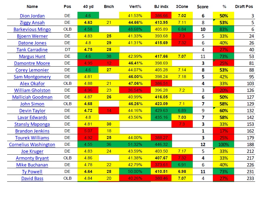
Combine measurable numbers play a significant role in how NFL teams rank players and construct their draft boards.   Of course, because player evaluation metrics are totally subjective, there is no way to know what one team values more than the next.  Here are the numbers for the prospects included in the defensive end group at the 2013 NFL Combine (“Pos” represents the position listed for each player on NFL.com):

(Note:  Because there is no Combine data for Jarvis Jones, who was drafted #17 overall by Pittsburgh, his data is not included in the analyses contained in this article.)

Ratios Used for Analysis

From the above data, the following measures can be calculated:

• Density calculated as weight in lbs/height in inches.  This permits us to normalize the differences in height and weight that naturally exist between players.  This number is best used to compare a player to his position average. Obviously, there will be players outside the average range (within 1 standard deviation) who are impactful players despite being heavier or lighter than the average.
• Vertical Jump to Height ratio (also, “Vert%).  The use of raw vertical jump results can be potentially misleading as the point of the vertical is to measure how much power one can generate, not so much how high one can jump off the ground.  This measure gauges the percentage of a player’s height he is able to jump off the ground, again, attempting to normalize.  The higher the better within that player’s position group.   
• Broad Jump Index (also, “BJI”).  This measure attempts to measure the “work” a player exerts during the drill to measure power generation (explosiveness).  Because a heavier man has a natural disadvantage, the broad jump is multiplied by the player’s Density, resulting in an index number.  Again, the higher the better within that player’s position group.   

Vertical to Height ratio and Broad Jump Index are graded to the group average along with 3 Cone, bench and 40 yard sprint times and players are awarded points as follows:

The total points earned are measured against potential points (some players did not perform all drills) for an overall score.  For example, Cornelius Washington had a 40 time of 4.55, (compared to 4.63 which is 1 standard deviation from the average) cranked out 36 reps on the bench (compared to 27.7), had the top Vert% of 51.32% and top BJI of 446.32 resulting in a perfect 12 points out of a possible 12 (I had no 3 cone number for him, so his max was 12, not 15 points).   Below are the scores for each Combine participant based on the performance metrics:

The combine performers with “passing grades” greater than 1 SD above average were Washington, Mingo, Powell, Hunt and Stuart.  While other factors go into the GMs’ player rankings, we would expect to see some correlation with draft position and combine performance.  Here is the table above sorted by draft position:

(Note: Walt Stewart was omitted from the list as he went undrafted due to medical issues.)

It is interesting to see that of the 5 first rounders analyzed, only one earned an “Exceptional” overall rating from our Combine analysis.  Two earned above average grades while two were below average.  Our top performer, Washington, didn’t get drafted until the sixth round. 

Fast Forward – 2015 Performance

So, ranking of the EDGE rusher group from the 2013 NFL Player Combine based on our analysis of participant performance did NOT match up very well with where the players actually went.  Athletic achievement at the combine didn’t translate into the high draft positions (and the higher salaries) these players had hoped they would receive.  Certainly, the NFL execs, armed with untold resources and scouting staffs of invaluable experience, have a leg up on fans and wanna-be scouts alike in this draft thing and knew something we didn’t.  The devil is in the details so there must be some method of interpreting the Combine data to which we average yokels will remain ignorant, horded by the NFL GMs.  Despite our unsophistication, let us attempt to close the loop on our exercise by adding player performance through the end of the 2015 season to the mix.   The list below was sorted by “Career  Sacks” for the sake of presentation (that is, there is no particular emphasis on Sacks for this exercise).

(Note:  Players with less than 3 career sacks were omitted from the list.)

Relative Productivity Metric

From a raw numbers standpoint, it would appear the Detroit Lions hit the jackpot with Ziggy Ansah.  He’s produced solid numbers anyway you look at them and is becoming a household name among the NFL faithful.  His numbers standout but how do we compare him to the rest of the field.   And how do we judge players who may have had a “redshirt” rookie year or have dealt with injuries (Washington )?  By comparing the above results to each player’s participation based on the total snaps played in 2015 (thanks to http://www.footballoutsiders.com/stats/snapcounts), we get a clear picture relative productivity.

Key:

• Tackles are calculated at 1 tackle for each solo and 0.5 for each assist.
• Snaps/Sack = The number of snaps played to generate one sack.
• S/S% = The percentage of player Snaps/Sack ratio compared to the group average.
• Snaps/T  = The number of snaps played to generate one tackle.
• S/T% = The percentage of player Snaps/Tackle ratio compared to the group average.
• Relative Prdctvty = Relative Productivity as the average of S/S% and S/T%.

From the table above, Armonty Bryant is clearly trending to be the most productive EDGE rusher selected in the 2013 NFL Draft.   His one sack every 35.27 snaps is nearly 10 times that of Okafor’s rate of one every 659 snaps.  Also, he produced one tackle every 5.71 snaps, nearly 12 times the rate of “Exceptional” combine performer and #6 overall pick Mingo. 

Here’s a final table showing our Combine grades, the draft positions and Relative Productivity side by side:

It must be acknowledged that there may be any number of unknown factors that may have impacted the final results of this analysis (players not reporting injuries at the Combine that hampered performance, depth chart issues limiting snaps, possible impact on how a player is used within a scheme or sub packages which could have provided some boost to stats, etc.).  Notwithstanding, the numbers would indicate the three player drafted lowest among the sample had the biggest impact despite only one having what could be considered an “Above Average” combine performance.

Outperforming Players

• Armonty Bryant (#1 Relative Productivity; Below Average Combine Performance, drafted 217^th overall), who attended DII East Central University in Ada, Oklahoma (anyone who can reply and identify what the East Central mascot is, without looking it up, will win a prize of subjective value!) , seems like the steal of the draft for the Browns.  But, (sorry CLE fans) this is the Browns we’re talking about. Bryant will miss the first 4 games of the season for violating league rules. It should be noted that back in college, Bryant sold drugs to an undercover cop and was subsequently arrested during practice. (http://www.silverandblackpride.com/2013/4/7/4192900/ecus-de-armonty-bryant-the-true-diamond-in-the-rough)   If it’s any consolation, despite being suspended for EIGHT games that year, he racked up 10.5 sacks and 54 tackles.
• Devin Taylor (#2 Relative Productivity; Above Average Combine Performance, drafted 132^th overall) played at the real USC where his impressive resume littered with team leading stats didn’t seem to make much noise to many, likely because  a kid named Jadeveon Clowney was the talk of the town.  Looking back at Taylor, he’s been a leader and winner at every level.  He and Ansah will be causing chaos for the Lions for years to come.
• David Bass (#3 Relative Productivity; Out of Range Combine Performance, drafted 233^rd overall) produced the highest tackle rate and the fourth highest sack rate despite playing the fewest snaps in the group (only 154 snaps).  He attended Missouri Western State (dreaded rivals of Kansas Eastern, I can only assume).  It’s clear why he wasn’t recruited out of school.  He was only a  three sport HS star and named to the All  Metro team in the competitive St. Louis area.  Who was elected captain of the football team.  And the basketball team.  Oh, did I mention he was captain of both teams his Junior AND Senior years?  He had 7 Passes Defended in his final college season as a Defensive End.  That’s as many as first round DB’s Eli Apple and more than Alexander Mackensie(5), Artie Burns (5) and Vernon Hargreaves (4).   Drafted by the Raiders, Bass is on his third team (he racked up 3 sacks in 8 games of action during the 2014 season for the Bears before he was cut), he will continue to provide depth to the Titans defensive line.

With some players moving to new teams and others looking to breakout and make names for themselves (not the least of which being the three named above), it will be interesting to see how the 2013 EDGE draftees perform in the upcoming 2016 season.    

2016 NFL Draft for Value Rankings

In every aspect of our lives, we're looking for value. 

Getting more for less. In the NFL Draft, it's all about taking advantage of the chaotic environment to find players other teams may have overlooked and avoiding the temptation to draft a player earlier than the market would dictate. This analysis attempts to use the expected position salaries from the first overall pick to the final man selected to assess the cost of each player compared to the potential value he may have to the franchise.

Assuming 2014 rookie salary figures for the recently drafted players (that is, Goff’s salary will be the same as the first player picked in 2014, Wentz's would be the same as the second player selected in 2014 and so on),  we can assume the value of a player to a franchise from a financial commitment level perspective.  This allows us to assume certain cost comparison values. Accordingly, Goff is 38.9x more costly than the last player drafted (please see the post for the Player Comparison Tool, which will allow you to compare players based cost comparison value).  Based on our reasoning, he is also 3.43x more valuable to his franchise than newly drafted Bronco Paxton Lynch.   So, if  Goff does not provide 3.43x more impact to his team, we could say the Broncos got a tremendous value in Lynch. Of course, the subjectivity of what is "impact" is material for another day, but this exercise is designed to help quantify an immeasurable value.  Remember, all figures relate to the #1 overall spot.  The higher the number, the lower the cost and the higher the potential for value. Using this comparative value concept as a framework for the rest of our analysis, we come up with the following three measures:

Average Overall Value/Overall #1 Pick – This measures the average value of each player’s comparable value to the Overall #1 pick.  Essentially, the higher the number,the lower in the draft the average player on that team was selected.  This number alone does not give us an idea of how well the Eagles selected because draft pick position is not an indicator of quality.  The Eagles were the top team with average picks at a cheap 27.9x less cost than the #1 pick. The Saints had the costliest picks, an average of 16.16x less than Goff.

Average Position Value/#1 – This measures each position player by their cost in relation to the #1 drafted player in their position.   For example, Joey Bosa was the #1 DE drafted so he has a value of 1.00x.  Shaq Lawson was the third DE to come off the board and, based on value to the franchise, Bosa is 2.86x more valuable than Lawson. If Bosa’s impact over the course of their rookie contracts is not 2.86x greater, the Bills got a tremendous value in Lawson. Going through each teams picks and comparing them to the player picked #1 at each position, the Niners got the best position value at 19.33x, while the Saints picked players early once their position “opened” after the #1 player was drafted, paying 4.17x

Average Sequential Pick Value – How soon after the last player  at a certain position was drafted did a team draft the same position?  In Rounds 2-7, if you select a position after it had just been selected, your value is going to be closer to 1.00x since salary values don’t decline as rapidly in these rounds as in the first. Big values can be found drafting outside of the current round.   For example, Kamalei Correa at #42 and Jihad Ward  at #44 are of nearly identical value coming out of the second round, but both are 2.02x more valuable than Carl Nassib, drafted in the top of the 3^rd round.  If Nassib performs on par with the other two, he was a major steel. The biggest gap (rightfully so in some minds) was at running back where Zeke Elliott is 6.55x more valuable than Derrick Henry.   The Titans got nice value with an avg of 1.67x when choosing the next position player while the Steelers seemed to be copy cats with an avg. sequential pick value of 1.03x.

Aggregate Draft Value – This calculated the average rank (1-32) in each of the three other categories. The Top 3 in terms of picking for value are the Niners, Eagles and Vikings.  The bottom three are the Saints (#32), Buccaneers (#31) and Panthers (#30).  To get the entire picture, we have to assess the quality of players they got at those perspective values.

Average Player Grade - Player grades were assigned based on the NFL.com DraftTracker  That Can Be Seen Here .  The teams with the highest average player grade were the Jaguars, Titans and Bears.  The lowest were the Patriots (#32), Chiefs (#31) and Eagles (30).

Best Draft for Value – Averaging the Aggregate Draft Value with the Average Player Grade give us the final Value Rank for each team.  The results are here:  Google Drive 2016 NFL Team Draft Value Comparison Final value grade is in the last column on the right. 

Art of the Deal – The four teams pulling off block buster trades had varied results.

• Titans – Traded out of #1 position had the 4^th best value based draft.
• Ram – Traded into the #1 spot and was 24^th on the list.
• Browns – Trade out of the #2 position and had the 28^th rated draft based on value.
• Eagles – Moved up to #2 and came away with the 14^th rated draft from a value perspective.

Rising in the East - The AFC East occupied the top 3 spots.

Southern Blues – Teams from the NFC South occupied 3 of the 4 bottom spots.

Most Picks

• CLE (14) – 28^th                    
• BAL (11) - 15th
• SF (11) – 7th

Fewest Picks

• CAR (5) -32^nd
• NO (5) -25^th       

Despite all the numbers and rationale, we won't know who "won" the draft until they line up to play in September.  As we go over this draft in three years, we will see who really got the best value out of this draft.  Usually, we'll know by which GMs and head coaches are still employed.  

2016 NFL Draft Comparison tool

Hello children,

I'm sure everyone enjoyed the NFL draft this weekend.  Talk about drama!  I'm working on a piece detailing who "won" the draft based on the actual "value" of each player to the franchise based on projected salaries. As a financial guy, I'm always measuring things in terms of the value of this compared to the value of that.  In a nutshell, if the first overall player selected is awarded salary "X" and you as a 3 round pick are awarded 1/10 X as a salary, then the #1 player has 10x more value to his franchise than you to yours.   On a team basis, this average Position Value figure is measured against the average player grade (using NFL.com for now).  As time goes on, we will be able to really judge the value of one player to another in general terms.

So, to whet the appetite, here is a spreadsheet that will allow you to compare the value of any one drafted player to another based on projected salary.  For example, Ezekiel Elliott is 6.55x more valuable than Derrick Henry.  That's a huge number especially for consecutively selected men playing the same position.

Here is the link to the spreadsheet:

 Boombear's 2016 NFL Draft Player Value Comparison Tool

Have fun with it and let me know if it bugs out on you.

Thanks.